Training Machine Learning Models using TrueFoundry's Jobs

Introduction

In this blog, we will introduce you to training machine learning models on the TrueFoundry Platform. We will discuss how we can run training jobs on TrueFoundry. We will also see how you can perform hyperparameter tuning easily for your machine-learning models, and run your jobs on GPUs.

Problem Statement

Let's first start with a problem statement, say we want to see how the diabetes disease will progress in a patient based on various features like age, BMI, blood pressure, etc. In this blog, we will train the Diabetes Dataset machine-learning model in scikit-learn.

Speaking of training machine-learning models, there are several ways to do so like training locally on your machine, training in Jupyter Notebooks, etc. However, the training process might require more resources than what is available on a local machine.

This is where TrueFoundry's Jobs enables you to deploy the training code to run on a remote machine and you can track the logs and metrics.

Note: While we are using this diabetes dataset, the instructions mentioned in this blog apply to other machine-learning / deep-learning models as well.

What is a TrueFoundry Job?

Jobs provide a way to run short-lived, parallel, or sequential batch tasks within the cluster. Jobs are designed to run to completion, rather than being long-running services or continuously running applications. Once a job is completed, compute and memory resources are released, hence we don't incur any extra cost.

Model Training Job on TrueFoundry

As said before, we will use the Diabetes Dataset in scikit-learn. The dataset contains 442 samples (patients) and 10 features, which are all numeric. The features represent various factors that can affect the progression of diabetes in patients. The target variable is also numeric and represents a quantitative measure of disease progression one year after baseline for each patient.

Set up Instructions

Before we proceed to train machine-learning models, let's go through the setup instructions:

Creating a Workspace

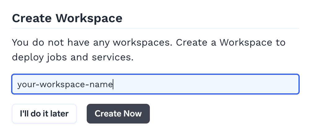
Go to the TrueFoundry Dashboard and create an account. As soon as you log in, you will be prompted to create a workspace. You would be deploying your jobs in this workspace.

Creating an ML Repo

Once you have created your workspace, go ahead and create an ML Repository from the dashboard.

An ML Repository is a collection of runs, models, and artifacts which represents a Machine Learning project. You can think of it like a git repository except that it houses artifacts, models and metadata. All the access controls can be configured on the level of ml-repo.

Adding ML Repo Access to your Workspace

Once the ML Repo is created, go to workspaces and edit your workspace and enable 'ML Repo Access'. Click on 'Add ML Repo Access' to add your ML Repo to this workspace. This will grant the job running in the workspace to write and read from the ML repo.

Install servicefoundry

pip install servicefoundry


Login to TrueFoundry

--host: Pass your TrueFoundry Dashboard URL here

sfy login --host <YOUR-HOST-URL-HERE>


Once we have completed the above setup instructions, we can move forward with the implementation section.

Implementation

Directory Structure

In this blog, we will adhere to the following directory structure where:

❯ tree
.
├── deploy.py
├── requirements.txt
└── train.py


Now let's go over the diabetes model training code:

Model Training Steps

Step 1: Import the required libraries

from sklearn.metrics import accuracy_score
from sklearn.datasets import load_diabetes
from sklearn.model_selection import train_test_split
from sklearn.compose import TransformedTargetRegressor
from sklearn.preprocessing import QuantileTransformer
from sklearn.svm import SVR


Step 2: Load the dataset

X, y = load_diabetes(as_frame=True, return_X_y=True)


Step 3: Split the dataset into training and testing sets

X_train, X_test, y_train, y_test = train_test_split(X, y, test_size=0.2, random_state=42)


Step 4: Create and train the machine-learning model

regressor = SVR(kernel=kernel)
model = TransformedTargetRegressor(
   regressor=regressor,
   transformer=QuantileTransformer(n_quantiles=n_quantiles, output_distribution="normal"),
)
model.fit(X_train, y_train)


Step 5: Make predictions on the test data

y_pred = model.predict(X_test)


Step 6: Evaluate the model's performance

accuracy = accuracy_score(y_test, y_pred)
print(f"Accuracy: {accuracy:.2f}")


Model Training Complete Code

from sklearn.metrics import accuracy_score
from sklearn.datasets import load_diabetes
from sklearn.model_selection import train_test_split
from sklearn.compose import TransformedTargetRegressor
from sklearn.preprocessing import QuantileTransformer
from sklearn.svm import SVR

def train(kernel: str, n_quantiles: int):
   # load the dataset and create train and test sets
   X, y = load_diabetes(as_frame=True, return_X_y=True)
   
   X_train, X_test, y_train, y_test = train_test_split(X, y, test_size=0.2, random_state=42)
   
   # initialize the model
   regressor = SVR(kernel=kernel)
   model = TransformedTargetRegressor(
       regressor=regressor,
       transformer=QuantileTransformer(n_quantiles=n_quantiles, output_distribution="normal"),
   )
   
   # train and test model
   model.fit(X_train, y_train)
   y_pred = model.predict(X_test)
   
   accuracy = accuracy_score(y_test, y_pred)
   print(f"Accuracy: {accuracy:.2f}"
   
   return regressor, model, X_test, y_test


Now that we have seen the code to train a machine-learning model, we can go ahead and learn about how to save (or log) such models for future use.

A Model comprises of model file and some metadata. Each Model can have multiple versions. We can automatically serialize, save, and version model objects by using the save_model_metadata method and the following are the steps to do so:

Model Logging Steps

Step 1: Import the required libraries

import mlfoundry


Step 2: Create an ML Repo Run

run = mlfoundry.get_client().create_run(ml_repo=ml_repo, run_name="SVR-with-QT")


A Run represents a single experiment which in the context of Machine Learning is one specific model (say Logistic Regression), with a fixed set of hyper-parameters. Metrics, and parameters (details below) are all logged under a specific run.

Step 3: Log Model Hyperparameters

run.log_params(regressor.get_params())


Step 4: Log Model Metrics

run.log_metrics({"score": model.score(X_test, y_test)})


Step 5: Serialize and Log a Versioned Model

model_version = run.log_model(name="diabetes-regression", model=model, framework="sklearn")
print("model_version =", model_version.version, "model_fqn =", model_version.model_fqn)


Each logged model generates a new version associated with the given name and linked to the current run. Multiple versions of the model can be logged as separate versions under the same name.

Model Logging Complete Code

import mlfoundry

def save_model_metadata(regressor, model, X_test, y_test, ml_repo):
   # create a run in truefoundry’s ml_repo
   run = mlfoundry.get_client().create_run(ml_repo=ml_repo, run_name="SVR-with-QT")
   
   # log the hyperparameters of the model
   run.log_params(regressor.get_params())
   
   # log the metrics of the model
   run.log_metrics({"score": model.score(X_test, y_test)})
   
   # log the model
   model_version = run.log_model(name="diabetes-regression", model=model, framework="sklearn")
   
   print("model_version =", model_version.version, "model_fqn =", model_version.model_fqn)


Now that we have seen the process of model training and logging, we can compile that into a single train.py file. The final contents of the train.py file should look like this:

train.py

# required import statements for both functions

def train(kernel, n_quantiles):
   ...

def save_model_metadata(regressor, model, X_test, y_test, ml_repo):
   ...

regressor, model, X_test, y_test = train(kernel="linear", n_quantiles=100)
save_model_metadata(regressor, model, X_test, y_test, ml_repo="YOUR ML REPO NAME")


This completes our code for model training and logging. Now we have to deploy the model training code as a job. The deploy.py contains the code for deploying the above model training code as shown below:

deploy.py

from servicefoundry import Build, Job, PythonBuild, LocalSource

# defining the job specifications
job = Job(
   name="diabetes-train-job",
   image=Build(
       build_spec=PythonBuild(command="python train.py", requirements_path="requirements.txt"),
       build_source=LocalSource(local_build=False)
   ),
)
deployment = job.deploy(workspace_fqn="YOUR WORKSPACE FQN HERE")


The requirements.txt should contain the following packages:

requirements.txt

pandas==1.3.5
scikit-learn==1.2.1
mlfoundry>=0.7.2,<0.8.0


In the above deploy.py code, a job is deployed that displays the accuracy score of the trained model in the logs when it is invoked. It also logs the trained machine-learning model. To do this, a job object is created using the servicefoundry.Job class. The job name is kept as diabetes-train-job here.

NOTE: Make sure you replace "YOUR ML REPO NAME" with your ML Repo Name in train.py and "YOUR WORKSPACE FQN HERE" with your workspace FQN in deploy.py file.

In the train.py file, you need to pass the Name of the ML Repo you created to the save_model_metadata() function. In the deploy.py file, you need to pass FQN of the workspace you created to job.deploy() function. Now execute the following command to deploy the job:

python deploy.py


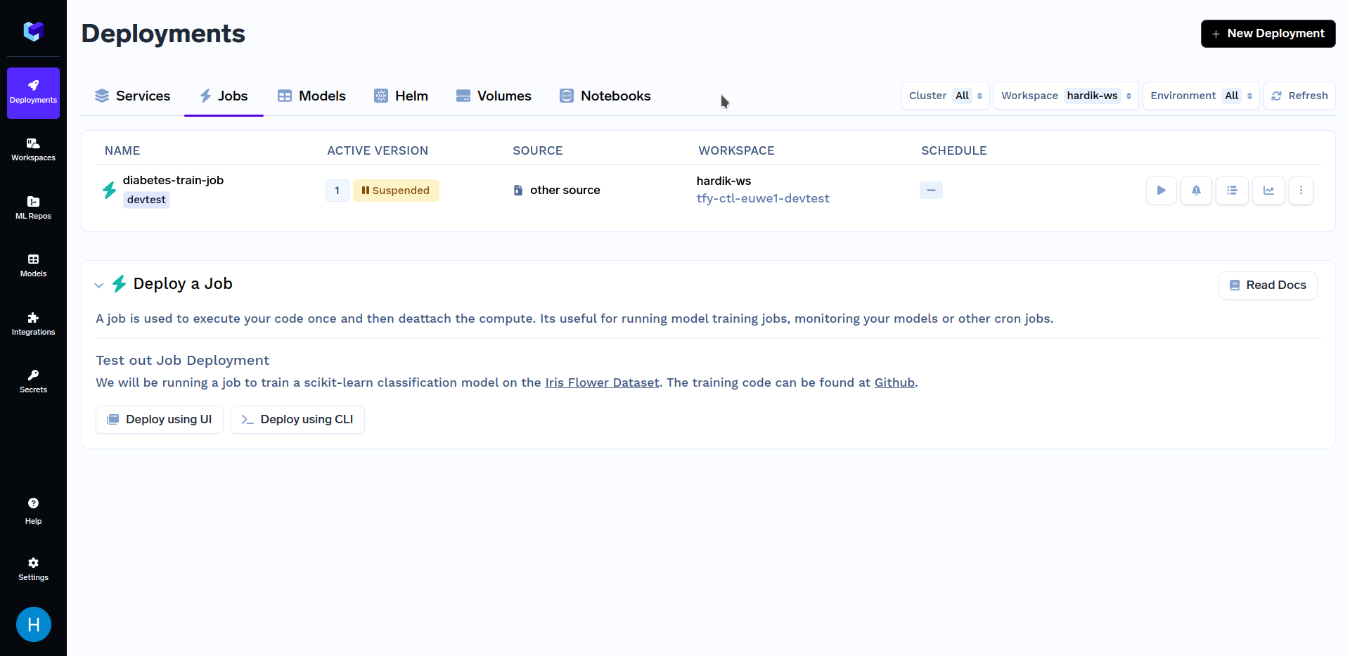
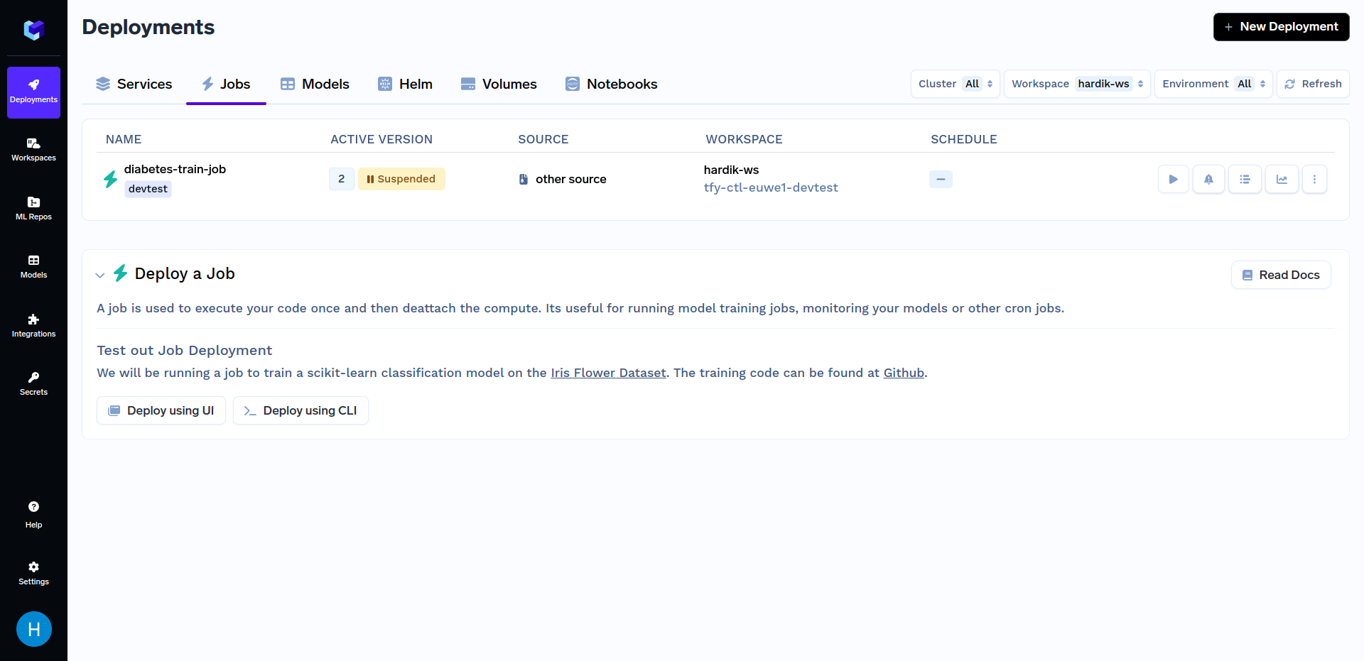
After deploying the training job, go to the "Jobs" sub-section in the "Deployments" section, it should look similar to this:

Now that we are done with deploying our job, we will want to trigger it. You can do so using either our Python SDK or the TrueFoundry Dashboard. Firstly, we will talk about triggering jobs from TrueFoundry Dashboard. To know about other methods of triggering jobs, refer to the Triggering Jobs from Python SDK section.

Triggering Job Runs from UI

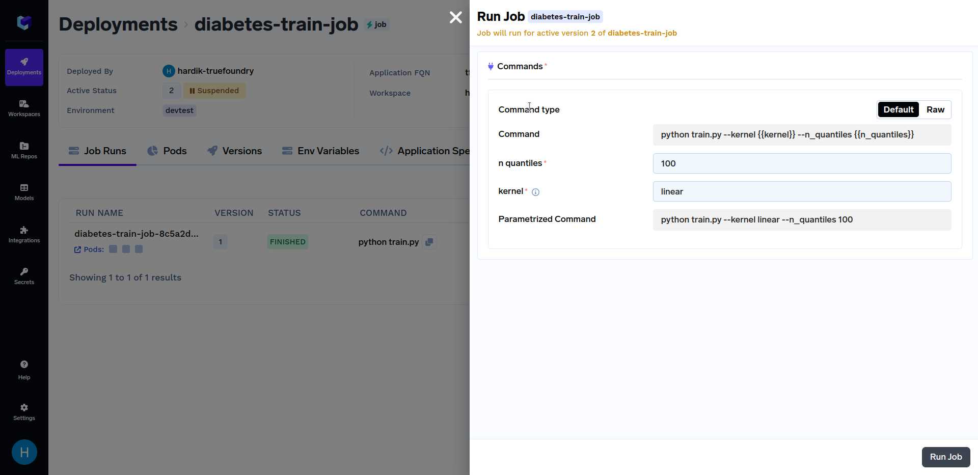
After the above training job has finished deploying, go to the "Jobs" sub-section in the "Deployments" section, click on the "diabetes-train-job", and click on the "Run Job" to configure the job before triggering. It should look similar to this:

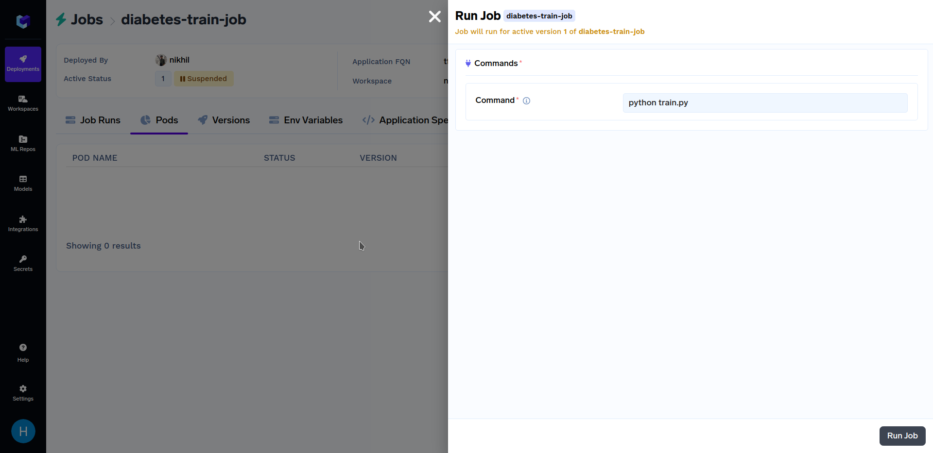
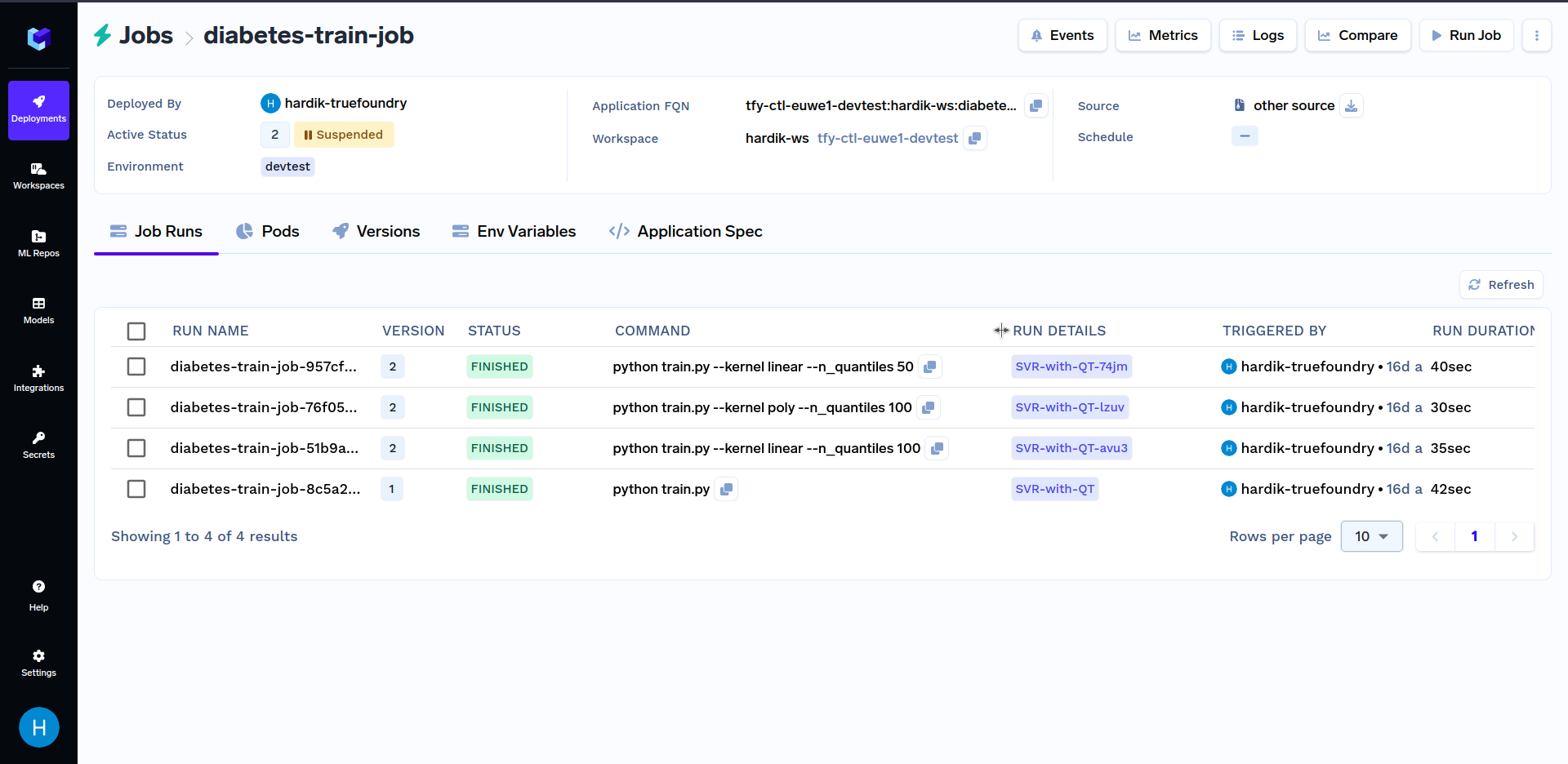
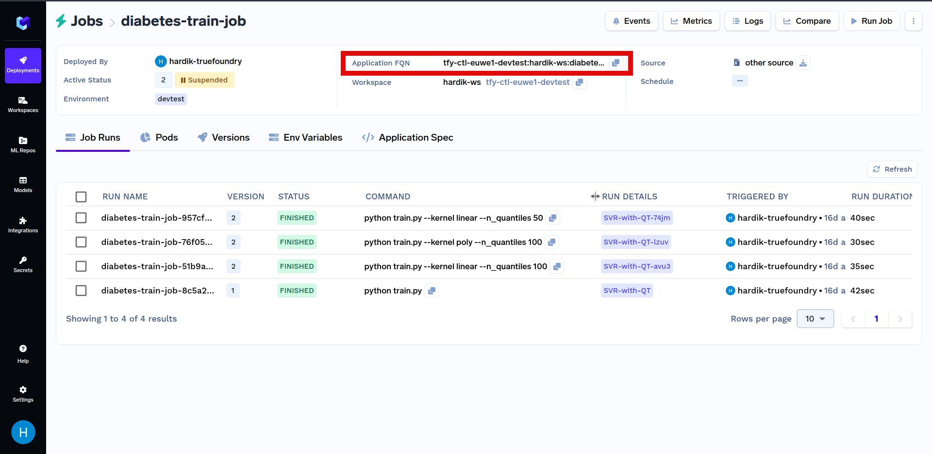
When at the above screen, click on "Run Job" at the bottom right corner to trigger this job. After the training job has finished running, go to the "Jobs" sub-section in the "Deployments" section, and click on the "diabetes-train-job", it should look similar to this:

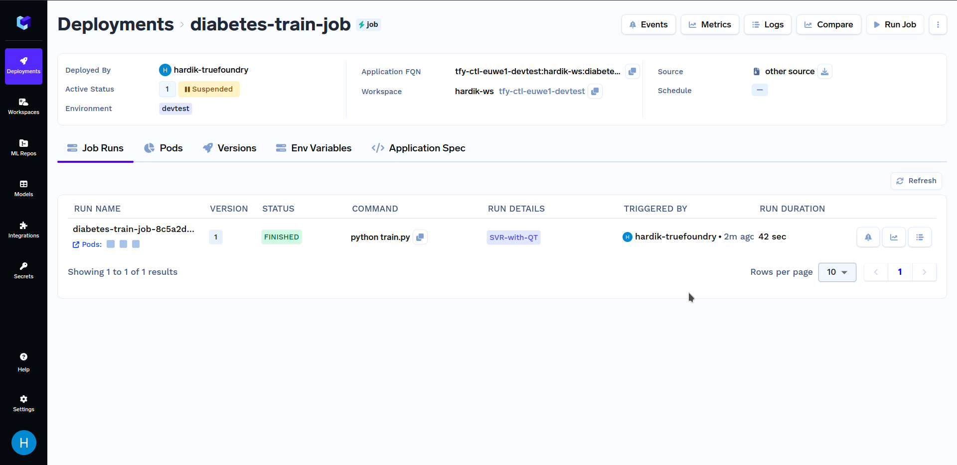
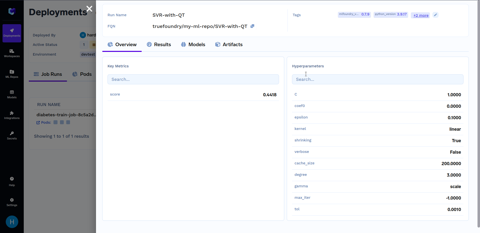
Under "Run Details", click on "SVR-with-QT" to see key metrics and hyperparameters that were logged in the train.py file. It should look similar to this:

Hyperparameter Tuning

Imagine that you have large-scale data processing or batch processing tasks where running a single job with different configurations is essential to not only streamline your workflow but also ensure consistency in job execution. In such cases, a Parameterized job will come in handy.

A Parameterized Job is a type of job that allows you to create multiple instances (pods) with different parameters or inputs. The primary goal of a Parameterized Job is to provide flexibility in job execution by customizing its behavior for different scenarios.

As an example, a job with command as python main.py --n_quantiles {{n_quantiles}} is a parameterized job as it takes n_quantiles as input before running. We can simplify the job deployed above using parameters.

To parse the command-line arguments, we will use the argparse module. The following code shows the updated code for the train.py and deploy.py files, where the default values of kernel and n_quantiles are linear and 100 respectively:

train.py

import os, argparse

def train(kernel, n_quantiles):
   ...

def log_model(regressor, model, X_test, y_test, ml_repo):
   ...

parser = argparse.ArgumentParser()
parser.add_argument("--kernel", default="linear", type=str)
parser.add_argument("--n_quantiles", default=100, type=int)
args = parser.parse_args()

regressor, model, X_test, y_test = train(kernel=args.kernel, n_quantiles=args.n_quantiles)
log_model(regressor, model, X_test, y_test, ml_repo=os.environ.get("ML_REPO_NAME"))


deploy.py

import argparse
from servicefoundry import Build, Job, PythonBuild, Param, LocalSource

parser = argparse.ArgumentParser()
parser.add_argument("--workspace_fqn", type=str, required=True)
parser.add_argument("--ml_repo", type=str, required=True)
args = parser.parse_args()

cmd = "python train.py --kernel {{kernel}} --n_quantiles {{n_quantiles}}"

# Defining the job specifications
# Only the command changes in 'image' attribute
job = Job(
   ...
   image=Build(build_spec=PythonBuild(command=cmd, ...), ...),
   params=[
       Param(name="n_quantiles", default='100'),
       Param(name="kernel", default='linear', description="svm kernel"),
   ],
   env={ "ML_REPO_NAME": args.ml_repo }
)
deployment = job.deploy(workspace_fqn=args.workspace_fqn)


NOTE: Make sure you replace "YOUR ML REPO NAME" with your ML Repo Name and "YOUR WORKSPACE FQN HERE" with your workspace FQN in the below command.

Now execute the following command to deploy the parameterized job:

python deploy.py --workspace_fqn "YOUR WORKSPACE FQN HERE" --ml_repo "YOUR ML REPO NAME"


Alternatively, you can execute directly from our Github repository.

git clone https://github.com/truefoundry/truefoundry-examples.git
cd training-job-example
python deploy.py --workspace_fqn "YOUR WORKSPACE FQN HERE" --ml_repo "YOUR ML REPO NAME"


Version 2 of the Job will be created after deployment has finished. After the training job has finished deploying, the next step is to trigger this job.

Click on the "diabetes-train-job", and click on the "Run Job" to configure the job before triggering. You can now change the n_quantiles and kernel parameters. It should look similar to this:

Try triggering job runs with different values of the kernel parameter like linear, sigmoid, poly and rbf. Similarly, you can use different values of n_quantiles parameters like 50, 80, 100, etc. Various job runs should look similar to this:

Comparing Job Runs from UI

You can compare the metrics of different job runs in the dashboard by clicking on compare button in the top right section of the dashboard as shown below:

You can read more about Parameterized Job Deployment here:

‍

Deploy a Job with Parameters

👍What you’ll learnCreate a training code with the option to pass hyperparameters as argumentsDeploying our training code as a job and adding the arguments as param This is a guide to deploy training code as a job via servicefoundry and pass different hyperparameters as arguments after deployment.Af…

TrueFoundry

‍

Triggering Job Runs from Python SDK

So far we have only seen triggering job runs from the TrueFoundry Dashboard. Now it is possible that triggering a job isn't always desirable via UI, so we will now go over how to trigger a job programmatically via Python SDK.

You can trigger your job programmatically by using the trigger_job function as shown below:

from servicefoundry import Job, trigger_job

# Configure a Job Deployment
job = Job(...)

# Deploy a Job
job_deployment = job.deploy(workspace_fqn="YOUR WORKSPACE FQN")

# Trigger/Run a Job
trigger_job(
 application_fqn=job_deployment.application_fqn,
 params={"n_quantiles":"80"}
)


It is also possible to get the application_fqn easily from the dashboard by going to Deployments --> Jobs --> Look for your job name in your workspace (here diabetes-train-job).

Below is another example of triggering a job programmatically. Firstly, replace YOUR_APPLICATION_FQN with the Application FQN of the job deployed above in the code shown below. The Application FQN for an application is highlighted below:

In the code shown below, we are randomly choosing a value for model parameters and triggering a job run using those parameters. After that, we search through job runs to find the run with the max score. The job run with the maximum score indicates a more optimal choice of model parameters.

import random
import mlfoundry as mlf
from servicefoundry import trigger_job

# Find deployed job, replace with the application fqn of your job
application_fqn = "YOUR_APPLICATION_FQN"

# Randomly generate params
n_quantiles = random.randint(50, 100)
kernel_values = ['linear', 'sigmoid', 'poly', 'rbf']
kernel = kernel_values[random.randrange(0, len(kernel_values))]

# Trigger/Run a Job
triggered_job = trigger_job(
   application_fqn=application_fqn,
   params={
       "n_quantiles": str(n_quantiles),
       "kernel": kernel
   }
)
print(f'Triggered job run with n_quantiles={n_quantiles} and kernel={kernel} and name as', triggered_job.jobRunName)

client = mlf.get_client()
ml_repo_name = "YOUR ML REPO NAME HERE"
runs = client.search_runs(ml_repo=ml_repo_name)

max_score = 0
for run in runs:
   metrics = run.get_metrics()
   print(f'All Metrics for run with name as {run.run_name}":', metrics)
   if 'score' in metrics:
       max_score = max(max_score, metrics['score'][0].value)

print("Model Max Score: ", max_score)


NOTE: Make sure you replace "YOUR ML REPO NAME HERE" with your ML Repo Name and "YOUR WORKSPACE FQN HERE" with your workspace FQN in the below command.

You can read more about Triggering Jobs here:

‍

Trigger a Job

👍What you’ll learnTriggering Jobs via Python SDK and TrueFoundry Dashboard This is a guide for triggering jobs via servicefoundry and...

TrueFoundry

‍

Comparing Job Runs from Python SDK

You can compare the metrics of different job runs programmatically by using mlfoundry.search_runs function as described in the following code:

import mlfoundry as mlf

client = mlf.get_client()
ml_repo_name = "YOUR-ML-REPO-NAME"

# Returns all runs
runs = client.search_runs(ml_repo=ml_repo_name)

# Search for the subset of runs with logged accuracy metric > 0.7
filter_string = "metrics.score > 0.7"
runs = client.search_runs(ml_repo=ml_repo_name, filter_string=filter_string)


You can read more about the search_runs function here:

‍

MlFoundry

module MLFoundry function get_clientInitializes and returns the mlfoundry client.Args: disable_analytics (bool, optional): To turn off...

TrueFoundry

‍

Deploy a Job utilizing GPU

Imagine dealing with large-scale models which have millions or billions of parameters. Training such models using traditional CPUs would be very time-consuming and may even be infeasible due to memory constraints.

For example, training a CNN model based on the CIFAR-10 dataset on a CPU environment with 10 epochs takes 36 minutes and 31 seconds, but the same model when trained on a GPU (NVIDIA K80) environment took only 4 minutes and 6 seconds. That is an improvement by a factor of 9x (Refer here)

GPUs play a vital role in large-scale model training. They provide the necessary memory bandwidth and parallel processing capabilities to handle large model sizes and complex architectures efficiently. Now we will go over how to use a GPU in a Job.

Using a GPU in the above example requires slight modifications in how a job is configured in the deploy.py file. The code below shows the updated Job Configuration for GPU utilization and Custom CPU and Memory resource allocation:

deploy.py

from servicefoundry import Job, NodeSelector, GPUType, Resources

job = Job(
   resources=Resources(
       # Configure GPU
       gpu_count=1,
       node=NodeSelector(gpu_type=GPUType.T4)
       
       # (Optional) Configure CPU and Memory Resources
       cpu_request=0.2,
       cpu_limit=0.5,
       memory_request=128,
       memory_limit=512,
   ),
   ...
)


Note: Rest of the code remains unchanged

Other Job Deployment Options

So far, we have seen several Job Deployment options such as image, params, and env. There are several ways to customize your job with advanced options. Some of those are as follows:

Set Trigger Type and Concurrency

Now that we have discussed Jobs that can be triggered manually either via TrueFoundry Dashboard or Python SDK. But what if we want a Job to run on a schedule (like a cron job)?

A cron job runs the defined job on a repeating schedule. This can be useful to retrain a model periodically, generate reports, and more. We can implement such jobs by changing their trigger type as follows:

from servicefoundry import Job, Schedule

job = Job(
   trigger=Schedule(
     schedule="0 8 1 * *",
     concurrency_policy="Forbid" # Values: ["Forbid","Allow", "Replace"]
   ),
   concurrency_limit=3,
   ...
)


For cron jobs, it is possible that the previous run of the job hasn't been completed while it is already time for the job to run again because of the scheduled time. In such cases, we may define concurrency_policy as follows:

1. Forbid: This is the default. Do not allow concurrent runs.
2. Allow: Allow jobs to run concurrently. Optionally, the maximum number of jobs to run concurrently can be changed by setting concurrency_limit to your desired value.
3. Replace: Replace the current job with the new one.

Concurrency doesn't apply to manually triggered jobs. In that case, it always creates a new job run.

Configure Retries

Job status can be of 3 types that are FINISHED, TERMINATED, and FAILED. A job can be configured to retry several times on failure.

A Job is marked as FAILED if it does not successfully finish even after the configured number of retries. Retries can be configured for a job like this:

from servicefoundry import Job

job = Job(
   retries=6, # default = 1
   ...
)


Configure Timeout

In some use cases, you may need to specify what maximum amount of time you want a job to continue executing.

Using timeout, you can specify (in seconds) the maximum amount of time for a job to run, whether it has failed or not. This will take precedence over the retries Limit. By default, this is set to 1000 seconds.

For example, if you set theretries to 6 and a timeout of 480 seconds, the job will terminate after 480 seconds regardless of how many times it attempted to run.

from servicefoundry import Job

job = Job(
   timeout=480,
   ...
)


Additional Job Deployment Options

Apart from the Job Deployment Options discussed in this blog, there are still some that we won't be discussing in this blog like:

• How to deploy a Job using a Pre-built Image?
• How to deploy a Job using a Dockerfile?

.... and a few more. You may refer to our Documentation given below to know the answers to the above questions :)

‍

Introduction

TrueFoundry is a platform on Kubernetes that makes it really easy to build, track and deploy models without having a detailed understanding of Kubernetes. Truefoundry is deployed on a cluster on your own cloud so that the data never leaves your environment and you don’t incur any data egress costs.T…

TrueFoundry

‍

Additional Examples

Our public repository truefoundry-examples contains this blog's job source code and it also includes several examples including LLM Finetuning, Getting Started with Notebooks, End-to-End Examples giving broader exposure to features offered by TrueFoundry Platform.

‍

GitHub - truefoundry/truefoundry-examples: This repository contains all the projects mentioned in the demo examples.

This repository contains all the projects mentioned in the demo examples. - GitHub - truefoundry/truefoundry-examples: This...

GitHub TrueFoundry

‍

Conclusion

In summary, TrueFoundry's Job provides a powerful framework for managing and executing training tasks in a scalable, fault-tolerant, and resource-efficient manner.

They enable you to distribute and control the execution of machine learning workloads, monitor their progress, and ensure that your training models are trained effectively and reliably, and this makes them ideal for executing one-time or on-demand tasks.